Bangla Character Recognition System — The Deep Learning way (2/3)

Welcome back, this post is the 2nd part of the series that Christina and I are working on as a part of our course project at Brown University, Data Science Initiative MS program. In the last post we discussed the data-set, the different classes and the distribution of the different targets.

In this article, we shall discuss the neural network architecture that we used for our project. But before we dive into that, here is a brief recap of where we ended last time.

We are trying to classify bengali handwritten letters into 3 targets — Grapheme roots, vowel diacritics and consonant diacritics. There are a total of 168 different sub-types of roots, 11 sub-types of vowel diacritics and 7 sub-types of consonant roots. Thing to note is that there is a massive imbalance as to the representation of each type in the training data, particularly in the class of grapheme roots. The training data comprise of scanned images of handwritten letters of sizes 137x236, but most of it was white spaces. Therefore we cropped, thresholded and de-noised the images to dimensions of 64x64, with the letters at the center. So now with the data primed for training, let’s look at the architecture.

What is a Convolutional Neural Network (CNN)

We assume that you know what the basic concept of a Neural Network¹ (NN) is. There are zillions of marketing descriptions of them but from a mathematical point of view, it is nothing a step by step procedure of mapping a input vector(s) to the desired output vector(s) through a series of affine transformations. The algorithm decides what those algorithms are (without human interaction, hence the word ‘machine’ learning) by passing known inputs and outputs to the network and then ask the computer to minimize a certain function (called loss function in ML terminology) to figure out which maps do a good job in reducing the error between the actual and the predicted outputs. We do this for a long time in an iterative fashion and we get (hopefully!) our generalized model. In our case, the input vector is a 4096 dimensional vector, since each image is 64x64 pixels, with each pixel having a value 0 or 1, based on whether it is a white pixel or black. On the output side, we have 3 of those of dimensions 168, 11 and 7 for grapheme root, vowel diacritic and consonant diacritic respectively.

However, while the more vanilla NN, also known as Fully Connected² (FC) networks have connections going from every input to every output vector component, the particular structure tends to look at every image as a whole to make the decisions. How’s that a bad idea? Well, confirm yourself that when you look at an image of a cat, the position of the cat with respect to the rest of image doesn’t matter in our judgement whether it’s a cat. Likewise, making decisions with the overall image sound like an overkill (and computationally unattainable) to go anywhere with that approach..

when you look at an image of a cat, the position of the cat with respect to the rest of image doesn’t matter in our judgement whether it’s a cat.

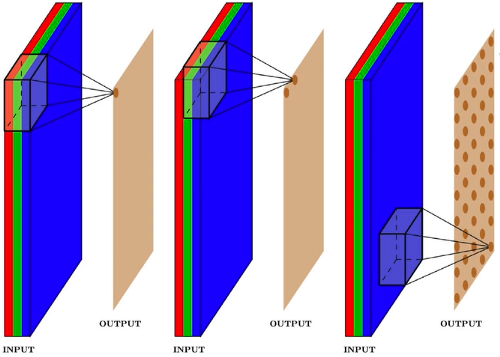
A CNN is a variant of NN where we attempt to preserve the aforementioned spatial invariance of our targets (cat/dog/vowels/consonants). Inspired by the human visual cortex, we slide a series of filters on our image and each of these filter pick up on a particular feature from the image that doesn’t depend on the absolute position of the feature in the overall image. To make it more concrete, imagine one of these filter, pick up long horizontal strokes, while some pick on vertical ones. We can also stack up these filters, to say one just picks up broad strokes which it then passes to subsequent filters that classify if that’s a horizontal or a vertical one. There is a fantastic article by Chris Olah where he explains CNN in much more details.

Densely Connected CNN or just DenseNet⁴

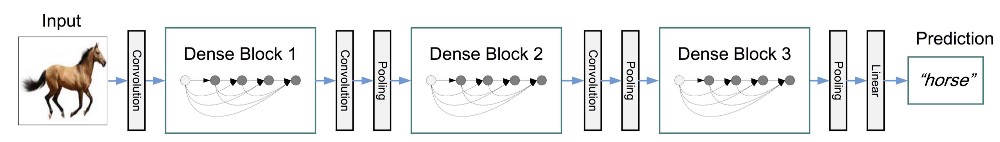
Unfortunately, a plain vanilla CNN also does not fit the bill sometime, due to the sheer complexity of the classification job. Going back to the example of strokes, merely isolating them wouldn’t be much help since a unique letter is a combination of a lot of strokes in different shapes. One way of alleviating this problem, is to give each filter the capability of identifying strokes while keeping it cognizant of all the inputs that were received at the previous layers while it does its processing. Here is an image of how that might look.

As you can see, the red line are the connections from the previous layer, and every successive layer has knowledge of the input to its preceding layers.

Due to hardware constraints of memory and computation power (we shall see later that these take a lot of memory due to the sheer no. of parameters involved), we cannot implement this in reasonable time-frame, even with the armament of GPU’s and compute times at Google or Facebook, let alone, a PC of a graduate student.

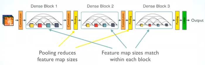
In mid 2016, Gao and colleagues came up with an architecture where instead of connecting the entire network, connectivity was done in chunks of layers (together called a Dense Block), which were connected to each other by a single convolutional layers and pooling layer⁵ (reason explained further down). At the end, we connect the output of the convolutional layers to dense output layers, which now just has to infer outputs from the convolutional layers response.

Nuts and bolts of DenseNet

A single dense layer can be broken in to 2 blocks:

Convolutional Block: This is the work horse of DenseNet. It’s major parameter is a growth rate, which determines the no. of filters in each convolutional layer. It is called growth rate, since when we concatenate the inputs, input to each layers is bigger by the amount of growth rate times the number of preceding layers.
Transition Block: Once we are at the output of a Dense Block, before it goes to the next layers, we pass it through another convolutional and pooling layer. This is so done because if you notice the output of each dense layer has a same size as that of the original input but since we have to downsample the next input as is standard in CNN architectures, we pass it through a (1x1) convolution layer and then an average pooling to achieve the desired dimensions.

Does it work?

DenseNet have been in the limelight for its comparable results to more complicated architectures such as ResNet or InceptionNet while reducing the no. of parameters and hence training time drastically. It also shares similar advantages of the fancier architectures such as alleviating vanishing/exploding gradient problems, and strengthening feature propagation and reuse. Below is a comparison with ResNet.

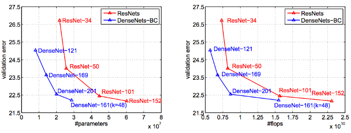
Comparison of accuracy between ResNets and DenseNets-BC (a variant DenseNet)

Observe how at the same level of accuracy, both the # of parameter and # of FLOPS are ~2–3x lower than ResNet.

It does suffer from the drawback that it takes a lot of memory while training since it has to keep track of all the preceding inputs inside the dense blocks.

Our Dense Net

Architecture

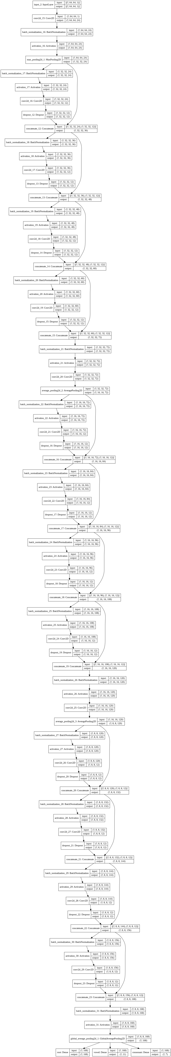
Coming back to the project at hand, here is our version of DenseNet (lovingly called SayanNet v4 :P )

https://ibb.co/HGtkwWs: Schematic of SayanNet v4 (also shown at the very end. It is huge.).

However the basic structure is as follows:

Input Layer — Input the images as 64x64x1 (since all images are grayscale)
(Optional) Augmentation Layer.
3 Dense Blocks — With 4 convolution layers each block, each convolutional layer having 12 filters. Followed by a transition block of average pooling layer (2x2 with strides of 2x2) for downsampling the output dimensions.
Global Average Pooling layer — To transform the final convolution layer output to a single vector
3 Output Dense Layers — For each target.
Several Dropout⁷ and Batch Normalization between convolution layers to reduce over-fitting and ensure signal strength.

In total we have:
Total parameters: 173,730
Trainable parameters: 170,802
Non-trainable parameters: 2,928

Other Hyperparameter

Optimizer — We used the Adam⁸ optimizer with a starting learning rate of 0.01

Loss function — Since each value is a label (with no numerical significance), we used the Sparse Categorical Cross-Entropy⁹ as out loss function for all outputs.

Metrics — Although the competition webpage measure on a weighted Recall metric, we use Accuracy¹⁰ as our training metric

Learning Rate — We used a variable learning rate, using TensorFlow’s native callback ReduceLROnPlateau¹¹ functionality on all 3 output losses. We started of with a learning rate of 0.01 and reduce by a factor of 0.2 each time the loss plateaus to a minimum of 0.0001.

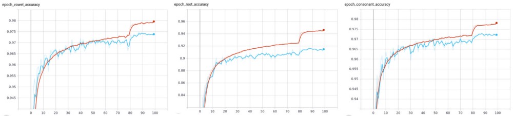
Preliminary Results

As mentioned before and the previous article, since our training data is imbalanced, we used scikit-learns train_test_split¹² function to do a class stratified split of the entire data-set into 90% training an 10% validation.

We trained the model with a batch size of 32 for a total of 100 epochs.

From left to right: Vowel Accuracy, Root Accuracy, Consonant Accuracy (Red — Training, Blue — Validation)

What's Next

Since we achieved success with just the base model with arbitrary parameters, the next step is to tune the hyper-parameters of the model, for improved results. Another thing to study would be the change in accuracy after adding a couple of dense layers before the output.

It is also interesting to see the effect of image augmentation during training to further reduce over-fitting and improved accuracy.

In the next post, we shall discuss in detail the result of the tuned network and make some attempt as to understand what each layer/block is extracting the features of the images to achieve the final result.

All codes for the project can be found in this github repository

References

Here is the full model

← Previous Post Next Post →