Disclaimer: I am not a epidemiologist. I do not understand much even within the wider gamut of Public Health. All I know is maths (the simplified versions at least), and this is an attempt to understand elementary models and then putting it through a probabilistic analysis pipeline to attempt to infer infection dynamics for personal sanity. The model and analysis is borrowed from a bunch of sources (citations at relevant sections). This is not close to real but only captures the broad trends obtained through drastic simplification and assumption albeit accurate within the bounds of those disclaimers.
Coronavirus disease 2019 (COVID-19) is an primarily respiratory disease caused by the severe acute respiratory syndrome coronavirus 2(SARS-CoV-2) that has brought the entire world to a standstill in an unprecedented manner than ever. The first confirmed case has been traced back to 17th November, 2019 in Wuhan, China$^1$. Since then, it has spread like wildfire across the globe. The World Health Organisation declared it as an public health emergency on 24th June, 2020 and a pandemic on 11th of March$^2$. As of June 24th, 2020, more than 9.23 million cases have been reported in more than 188 countries, resulting in more than 476,000 deaths$^3$.
I'm certain that you are more than just aware of the severity of this disease and how it might have permanently changed the trajectory of human civilisation. Masks might become the next fashion item and 'zooming' and 'social distancing' have already become an inherent part of our daily vocabulary. The death, suffering and economic hardships faced by mainly the elderly in the age demographic and the economically marginalised segments of the society has been exacerbated beyond controllable measure. Things are gloomy for real.
However, you have the news for that. I want to talk about things that are more personal. While the world quarantined indoors, we got the chance to introspect on those affairs that are otherwise put in the back-burner behind the race of finishing work-deadlines, business trips, office parties, EDM concerts and etc. etc. A lot of folks re-discovered the value of family while some finally learnt to use the grill that was bought on a last minute impulse at a black-Friday sale 3 years ago.
I'm tired though. Winter is gone. Summer is here and while I am fortunate enough that my family and circle of friends have all overcome the set-back, tension and turmoil or the past few months, I really want to get back to the good old days. Mirroring the same feeling, places have started to open-up again. Some countries are also slowly opening up national (and international) transportation systems. Pretty soon things would be 'back to normal'.
That begs the question - Is it safe to resume public activities again? Have we really 'flattened the curve'. What exactly is that curve anyway? Certainly, there are still daily new cases being reported everywhere. This article is an attempt to try to understand basics of a mathematical framework that can guide our intuitions. First, we shall discuss briefly a deterministic mathematical model of the spread of an infection to establish the relationship between different quantities that define the spread of infection. In other words, we shall talk about a simplified SIR (Susceptible-Infectious-Removed) model, and then use existing data to build an estimate of parameters via a probabilistic approach that can help us guide us to the decision - 'Is it safe to go the Gym? (Or parties!! while we are at it)'
Deterministic SIR Model$^4$
The SIR model compartmentalises individuals to 3 categories:
- Susceptible - Members of the population that are healthy now but can be infected
- Infectious - Members of the population's that are already infected and thus can spread the disease to other susceptible members.
- Removed - Members who have recovered, had previous immunity or are dead. A recovered person can neither spread the disease nor can get infected.
The forthcoming calculation is severely simplified but gathers the interesting trends which an infectious disease charts as it spreads through the population.
Let's begin with a population of $n$ total individuals. All of whom are susceptible to the disease. At time $t = 0$, let's assume we have $1$ infected person and therefore $n-1$ susceptible person. Let us also say that the probability of the spreading of the infection by a particular infected individual to another susceptible individual is $p$. Therefore it is straightforward to say that in the next day there would be $i_1 = p(n-1)$ infected persons, $s_1 = n-1 - p(n-1)$ susceptible individual and say that the 1 infected individual from yesterday is by definition removed from the population ($r_1 = 1$). It might sound absurd that if $p$ is not an integer, how can we have fraction of individuals that are sick, but mind you, this is only an 'average' number. So it's OK.
However a bigger concern is the time-step of 1 day. It is too coarse. Even more importantly, the assumption that each infected person remains infected (thus capable of spreading the infection) for just 1 day is really absurd. So let's address that with the help of differential equations.
Change in the no. of susceptible people in a time-gap of $\Delta t$ $$ \begin{equation*} S_{t+\Delta t} - S_t = -pS_tI_t\Delta t \end{equation*} $$ where $S_t, I_t$ are the no. of susceptible and infectious people at time t. Note that the no. of susceptible people is monotonically decreasing for a given fixed population size. Hence the chnage has the -ve sign associated with it. Let us also recast our transmission probability p in terms of the population, hence $$ p = \frac{\beta}{n}$$ where $\beta$ is the contact-rate which gives the no. of transmission per infectious person earlier on in the disease life cycle (when $S_i \approx n$) $$ \begin{equation*} \Delta S_t = -\beta\frac{S_t}{n}I_t\Delta t \end{equation*} $$
The change in the no. of infectious people can be given by the no. of susceptible individual who got infected at the previous time step as well as the no. of people who got infected in some previous time step and are still infectious (called serial interval). $\gamma$ in our calculation is therefore in units of (time)$^{-1}$ and is the reciprocal of the serial interval. In the case of COVID, the serial interval is about 4 days$^5$ $$ \begin{align*} I_{t+\Delta t} - I_t &= \left(\beta\frac{S_t}{n}I_t - \gamma I_t\right)\Delta t\\ \implies \Delta I_t &= \left(\beta\frac{S_t}{n} - \gamma\right)I_t\Delta t \end{align*} $$
Finally, the no. of removed individuals are: $$ \begin{equation*} \Delta R_t = \gamma I_t\Delta t \end{equation*} $$
Recasting the equations with $\Delta t \to 0$, we get $$ \begin{align*} \frac{dS}{dt} &= -\beta\frac{S}{n}I\\ \frac{dI}{dt} &= \left(\beta\frac{S}{n} - \gamma\right)I \end{align*} $$ Note. that $S+I+R = $ constant. Hence we never have to explicitly calculate the third variable (at least in this simplified set-up)
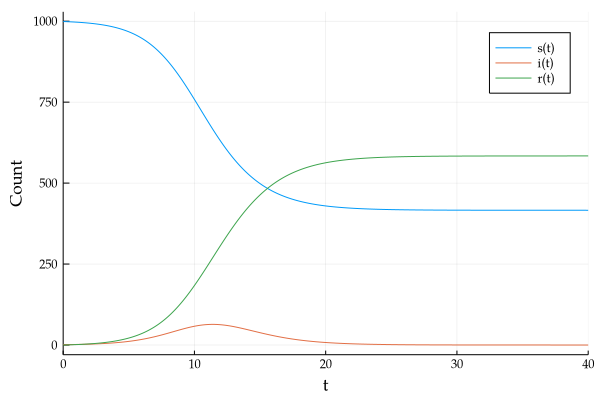
Running a small simulation, with $\beta = 1.5$, $n = 1000$ for 40 days gives us the following curve.
If we re-plot this with $\beta = 2.0$, and focus only on the infectious curve, we see
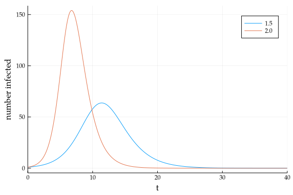
It is this bell-shaped infectious population curve that is source of the buzzword - "Flatten the curve", which is another way of stating the reduction in the infection transmission rate. (Greater 'flatness' of the curve is equivalent to lesser person-to-person spread of infection on average)
Revisiting the Infection curve
Lets us look at the infection rate equation once again.
$$ \begin{equation*} \frac{dI}{dt} = \left(\beta\frac{S}{n} - \gamma\right)I \end{equation*} $$Based on the above equation, we can see that when $\beta\frac{S}{n} - \gamma > 0$, we have growth, and vice versa. $$ \begin{align*} \beta\frac{S}{n} - \gamma &> 0\\ \text{assuming onset of epidemic, so } & S \approx n\\ \underbrace{\frac{\beta}{\gamma}}_{R_0} &> 1 \end{align*} $$ This shows what we already knew from popular media, R$_0 > 1$ means infection is spreading exponentially through the population, while R$_0 < 1$ indicate the opposite.
Another way to understand what R$_0$ represents is by considering that since we have 1 infectious person infecting $\beta$ individuals per unit time for a total of $\frac{1}{\gamma}$ time units, then no. of infections spread by one infectious person on average (R$_0$) is given by $\frac{\beta}{\gamma}$
We can also connect a more general quantity R$_t$ with R$_0$, by observing, R$_t$ $\propto$ S$_t$, and R$_t$ = R$_0$, when $t = 0$, therefore $$ \begin{equation*} R_t = R_0\frac{S_t}{n} \end{equation*} $$ R$_t$ can be interpreted as a generalised R$_0$ on any given time points than the first day of infection in the population (or other grave assumptions of R$_0$ being constant over time).
Therefore we get, $$ \begin{align*} \frac{dI}{dt} &= \left(\beta\frac{S}{n} - \gamma\right)I\\ \implies \frac{dI}{I} &= \gamma(R_t - 1)dt\\ \therefore \log I_{t+\Delta t} - \log I_t &= \gamma(R_t - 1)\Delta t \end{align*} $$ However we have data of cumulative confirmed infections (which is basically a reducing list of the number of susceptible person), instead of tracking data for each infected individual from the onset. Hence we could relate R$_t$ with the cumulative number of cases till day T by tracking the change in a small interval $[T, T + \Delta T]$ $$ \begin{align*} T_{t+\Delta t} - T_t &= \beta\frac{S_{t+\Delta t}}{n}I_{t+\Delta t}\Delta t\\ &= \beta\frac{S_t}{n}I_t\exp\big[\gamma(R_t - 1)\Delta t\big]\Delta t \end{align*} $$ While on the interval $[T - \Delta T, T]$ $$ \begin{align*} T_t - T_{t-\Delta t} &= \beta\frac{S_{t}}{n}I_{t}\Delta t \end{align*} $$ Thus we can calculate the diff (difference of consecutive pair) and then from the result of the operation, again divide each consecutive pair. The quantity thus obtained can be directly related to R$_t$ as per the equation: $$ \begin{equation*} \frac{T_{t+\Delta t} - T_t}{T_t - T_{t-\Delta t}} = e^{\gamma\Delta t(R_t - 1)} \end{equation*} $$
Herd Immunity
Before we delve into estimation of the above discussed parameter R$_t$, here is a brief digression to discuss a concept of herd immunity. The underlying concept lies in the fact that if the disease spreads rapidly throughout the population, such that a major fraction is already infected or removed from the susceptible population, then effectively these people form a sort of barrier protecting those who are still susceptible. This is due to the fact that with increasing non-susceptible population, the probability of a susceptible individual coming in contact with an infectious one become rarer. Imagine, the removed population creating a shield around the susceptible ones protecting them from the infection.
The fraction of population that is to be infected or removed before herd immunity kicks in can be calculated by once again observing the infection rate equation. $$ \begin{equation*} \frac{dI}{dt} = \left(\beta\frac{S}{n} - \gamma\right)I \end{equation*} $$ By definition we are looking for that point where the rate of infection switches from +ve to -ve, or in other words, when $\frac{dI}{dt} = 0$, $$ \begin{align*} \beta\frac{S}{n} - \gamma &= 0\\ \implies \frac{S}{n} &= \frac{\gamma}{\beta}\\ &= \frac{1}{R_0} \end{align*} $$ Hence, the fraction of the population that has to be removed or infected before the rate of infection starts to decrease due to herd immunity (also known as Herd Immunity Threshold, HIT) is given by $$ \begin{align*} 1 - \frac{S}{n} &= 1 - \frac{1}{R_0}\\ \text{HIT } &= 1 - \frac{1}{R_0} \end{align*} $$
Note, that this includes that since this included infectious and removed, we could ensure herd immunity without mass-spread infection by increasing the number of initial removed population (i.e. by vaccination).
Bayesian Estimation of R$_t$$^6$
In the last section, we derived a relationship between the daily record of cumulative cases and R$_t$. It is wise to reiterate at this point that the quantity R is the measure of if the infection in spreading in the population (R$_t > 1$) of is gradually dying out (R$_t < 1$). To be able to predict its behaviour over time also gives us the ability to guide policy such as the safety of reopening and the associated preparedness for a second wave (if any).
The approach that follows is taken from a modified approach to Bettencourt and Ribeiro 2008, the gist of the approach is as follow. Instead of trying to deterministically obtain R$_T$, we assume that it has a certain underlying distribution. Now we know intuitively that although it is rare for a particular infectious individual to pass on the virus (reducing contact), there are lot many of them, hence the 'average' number of infections caused by a single infectious individual is not negligible. The classical distribution governing such behaviour is known as the Poisson Distribution.
A Poisson distribution is a single parameter discreet probability mass function. The parameter is also the mean of the distribution. Hence, let us define $\lambda = k_t e^{\gamma(R_t - 1)}$ where $k_t$ is the increase in the number of cases today, and assign it as a Poisson distribution. Hence, given we expect to see $\lambda$ new cases on average each day, the actual no. of new infection on any given day is given by $$ P(k|\lambda) = \frac{\lambda^k e^{-\lambda}}{k!} $$ which would be around the expected mean value but slightly deviated by a smaller number.
However, out target is to find $P(R_t|k)$, i.e. given all the previous data, what is my R$_t$ in the following days within certain bounds of confidence. For this we can employ Bayes Theorem. $$ P(R_t|k) \propto P(k|R_t)P(R_t) $$ To use this formulation to zero-in on the most likely value of R$_t$, we assume a prior distribution ($P(R_t)$) that R$_t$ might have. We then calculate the probability of seeing the data for the day ($P(k|R_t)$) under the prior parameter. This is known as the likelihood function. We could then apply the above Bayes formula and normalise the resulting distribution so that it sums to 1, This new probability function is called the posterior which gives us a better estimate of the true parameter. We then sample from the posterior ($P(R_t|k)$), next days value of R$_t$ (which is now the prior of day 2) and repeat. This iteration in the long run enables us to identify the true $\lambda$ and thereby R$_t$
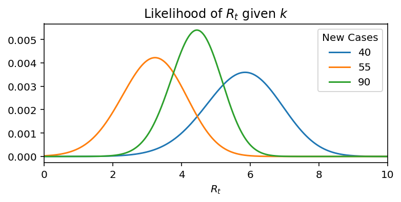
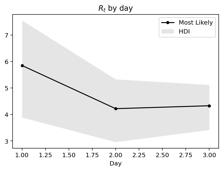
Lets make this idea more concrete with the help of a toy example. Assume, the new infections for 4 days: 20, 40, 55, 90. If we take each day independently, then the distribution of R$_t$ is as:
But if we do Bayesian updates, then in each successive day we incorporate information of all previous days, hence we get:
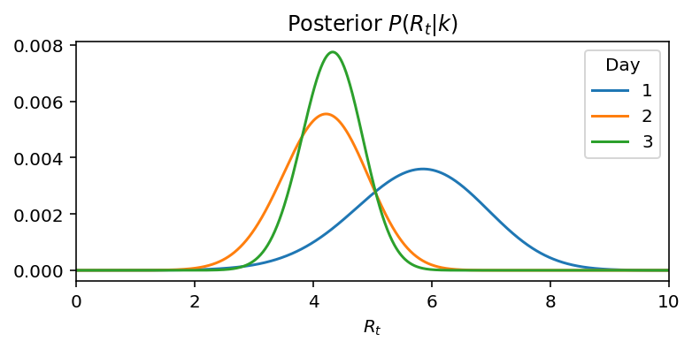
We can see, that on day 1, the mean was about the days record of new cases. On day 2 and day 3, in the light of new information, the mean is switching much less and more importantly is getting narrower implying greater confidence over the prediction We could also observe this increase in confidence by observing the narrowing of the 95% confidence intervals.
.
Application to Real Indian data
All data was obtained from https://api.covid19india.org/
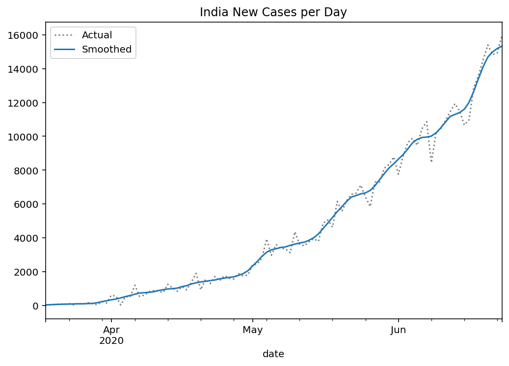
Since the data reported regularly is noisy due to mistakes, backlogs etc., we first apply a Gaussian filter to the data (or any other filter that can noise in the report). Following the data smoothing, the daily new cases per day is:
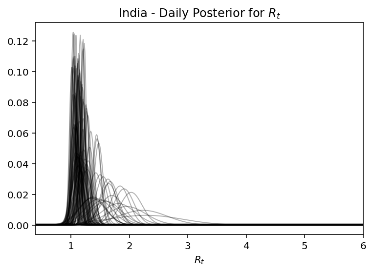
Running the machinery described above, we can observe how the posterior narrows with more time
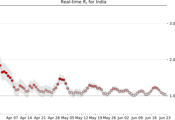
Therefore the Real time R$_t$ prediction of India is:
Likewise the $R_t$ prediction for some other Indian states are:
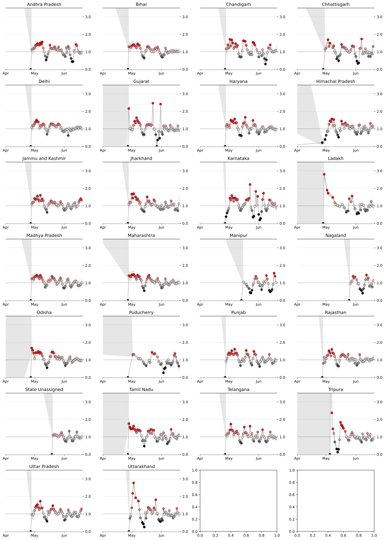
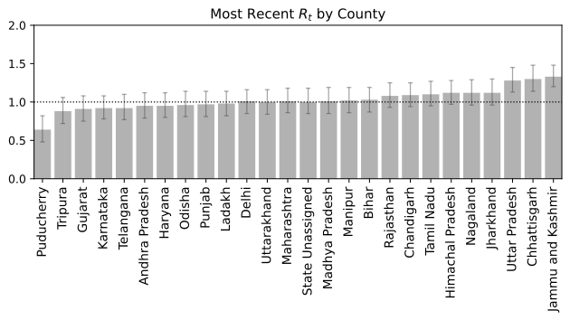
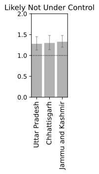
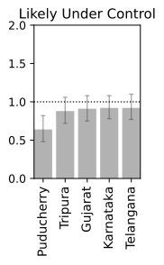
Based on this we could also predict which states are doing well and infection is reducing which which states are far from being in a stable conditions.
Closing Thoughts
We now have a basic framework to merit the current status of a location provided we have sufficient past data. Irrespective of the global scenario and absolute numbers which can be deceiving without associated information of density and local record, a real time R$_t$ information is more suited for making personal decisions of public interaction. Note, that the analysis is probabilistic and suffers from the assumptions that may not be in tune with the real dynamics. It also depends on past data, and while we are at the tail-end of a infection curve, slight variations can make or break the calculation. Just because R$_t < 1$ right now, does not mean that we can carelessly venture out since one super-spreader can quickly pull up the numbers very quick. Also, you can be just unlucky to be in close contact with an infectious person irrespective of mean trends. Specially in a crowded place like India, re-opening at a phase where the R$_t$ is still hovering close to 1 is certainly not safe. Let this post guide your intuition but not suggest that all is well. Hold on to those masks and social distancing norms for a few more days. We are almost there. Hope you had an informative read. Have a good rest of your day.
I would like to thank Dr. Sam Watson of Brown University, Data Science Initiative for motivating me to write this post. The material discussed here is borrowed from his Data Gymnasia course on Mathigon and his lecture series here in the university. Both Sam and I therefore owe the Bayesian analysis code from Kevin Systrom, founder of Instagram and manager of rt.live. Sam also acknowledges Tom Britton of Stockholm University for ideas about the stochastic SIR model that has not been mentioned here but whose average statistic is explained through a deterministic model. My personal contribution is to calculate the R$_t$ estimate with the data for the republic of India and its states.
Useful Links
- UVAs Biocomplexity Institute dashboard shows the geographic spread of the virus over time.
- 3Blue1Brown presents a video narration examining the effects of various agent-based simulation features.
- Gabriel Goh provides a simple, elegant calculator for illustrating how parameter changes affect trajectory of the infection curve.
- Kevin Simlers blog post introduces and discusses quite a few manipulatives for varying simulation parameters.
- The COVID-19 Forecasting Project gives estimates for current numbers of active cases as well as projections for the future.
- COVID Projections is another forecasting site with positive reviews from experts.
- rt.live tracks US state-by-state estimates for the current reproduction number (R$_t$) over time.
Here are some data sources for self-exploration:
- Singer tap is The most exhaustive data tap on COVID-19 provided by https://www.singer.io/
- The Johns Hopkins data is perhaps the most canonical source on global COVID-19 data.
- The COVID Tracking Project includes data on negative tests as well positive ones, but it only covers the United States.