Generative Adversarial Networks — Smearing the gap between real and fake

A general assumption of Machine Learning (ML) is that everything in this world has a distribution associated to it. This distribution can be formally described as a weighted sum of a pre-defined set of features, and it is the weights that differentiate one thing from another. One expects that although the range of permissible weights for each feature is, in principle, unbounded, it is mostly concentrated around a particular mean, separated by a well-defined standard deviations.

As an example, we can think of all humans being samples from a distribution where the set of features are — colour of the skin, height and shape of the nose (just to name a few). Some tend to have sharper nose, others have different skin tone, some are short while others are tall. However the range of values across all those features do happen to be centred around a mean differentiated by small deviations. (We really don’t have pink colour skin and fortunately vampires don’t exist, or do they?)

Now if the task is to just generate more humans faces we could go about it in roughly two techniques — We could attempt to find the exact distribution of humans — i.e. what is range of human brain sizes, human canines etc. OR we can choose to not deal with explicitly modelling the distribution but just be able to sample from the locale of human faces in the aforementioned feature landscape.

The latter technique of sampling from a distribution without explicitly modelling the distribution is what is known as ‘Direct Generative Modelling’, and GAN³ is the state-of-the-art direct generative modelling deep learning technique that leverages a neural network architecture and optimisation schemes to learn the function which converts arbitrary noise input to a convincing sample of the image space.

In this article, we shall look at GANs — first in a descriptive way where we try to get an intuitive notion of the technique and how it is implemented by a neural network in a black-box sense. Then we shall formalise the qualitative description a more mathematics one and conclude with a hand-wavy proof of how the GAN algorithm effectively lets us sample from the unknown intractable distribution.

GAN — The Game Theoretic Neural Network

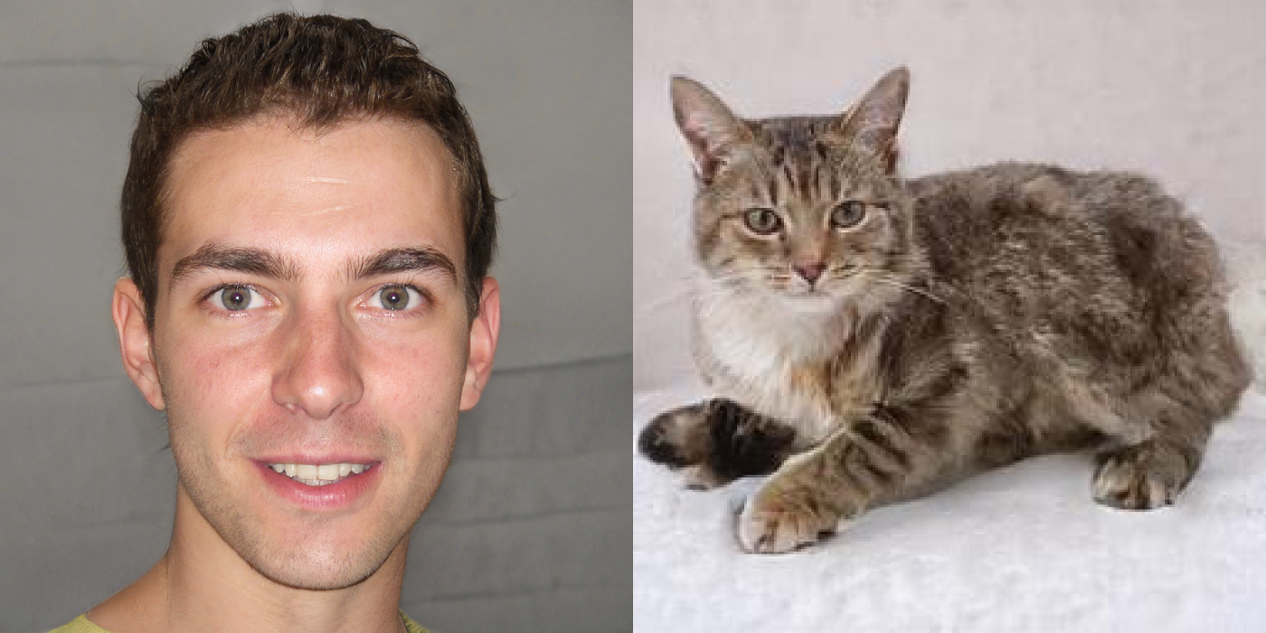
As the name suggest, GAN is a combination of 2 networks — the Discriminator and the Generator. The Discriminator is basically a binary classifier that is trained to distinguish ‘real’ samples ( real human images captured on a camera) from ‘fake’ ones (images generated by the network). The Generator is the other network that generates those fake images (from noise) that our Discriminator learns to classify from the real ones.

The key idea behind GAN is the game-theoretic approach of training where the discriminator and the generator compete against each other (they are adversaries/enemies) and try to beat each other in a zero-sum non-cooperative game-theoretic sense. This means that during training, the discriminator gets better and better at separating out the real from fakes while the generator, seeing how good the discriminator is getting, learns to improve its fakes to fool the generator. Thus in a figurative game of tug-of-war, the discriminator keeps improving but the generator always plays catch-up and ends up generating more convincing fakes with each training epoch till both the players reach a Nash equilibrium.

Let’s see this play out in a simple one-dimensional space.

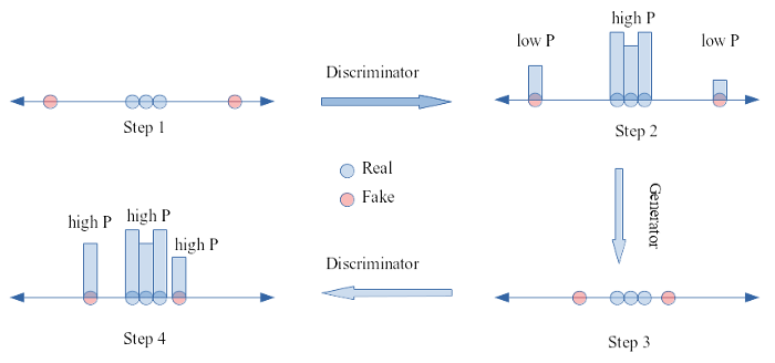
Step 1. The generator generates samples.

Step 2. The discriminator learns on both real and fake and assigns a lower probability to the fake data.

Step 3. Noticing how the discriminator behaves, the generator generates new sample closer to the real ones.

Step 4. The discriminator does get better, but the difference of probability assigned to real and fake reduces

Envision this going on-and-on in a round-robin fashion, where the generator finally learns to generate samples so close to real that they are virtually unresolvable.

Architecture and Tensorflow implementations

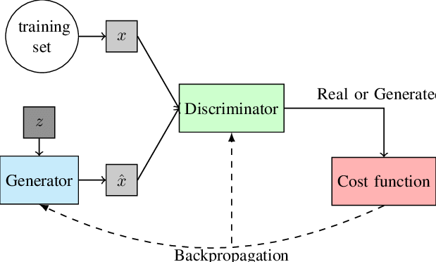
As explained before, we see two networks

• Generator — which takes as input a latent variable (usually a lower dimensional vector, usually sampled from a multivariate gaussian of mean 0 and standard deviation Σ) and generates an image.
• Discriminator — which takes as input the fake and real images (each labelled appropriately) and outputs a binary variable (0 for fake, 1 as real)

The training goes as:

  
  for no. of epochs do
     for no. of training samples do
        * sample minibatch of m noise samples {z₁,...,zₘ} from noise prior p(z)
        * sample minibatch of m real samples {x₁,...,xₘ} from real data
        * Update the discriminator by backpropagating wrt to loss function (keeping the generator fixed)
        * sample minibatch of m noise samples {z₁,...,zₘ} from noise prior p(z)
        * Update the generator by backpropagating wrt to loss function (keeping the discriminator fixed)
  

Let us see a tensor-flow implementation⁴ of the network.

# generator takes noise (a random coding) and generates FMNIST images
generator = keras.models.Sequential([
    keras.layers.Dense(7 * 7 * 128, input_shape=[codings_size]),
    keras.layers.Reshape([7, 7, 128]),
    keras.layers.BatchNormalization(),
    keras.layers.Conv2DTranspose(64, kernel_size=5, strides=2, padding="SAME",
                                 activation="selu"),
    keras.layers.BatchNormalization(),
    keras.layers.Conv2DTranspose(1, kernel_size=5, strides=2, padding="SAME",
                                 activation="tanh"),
])
discriminator = keras.models.Sequential([
    keras.layers.Conv2D(64, kernel_size=5, strides=2, padding="SAME",
                        activation=keras.layers.LeakyReLU(0.2),
                        input_shape=[28, 28, 1]),
    keras.layers.Dropout(0.4),
    keras.layers.Conv2D(128, kernel_size=5, strides=2, padding="SAME",
                        activation=keras.layers.LeakyReLU(0.2)),
    keras.layers.Dropout(0.4),
    keras.layers.Flatten(),
    keras.layers.Dense(1, activation="sigmoid")
])
gan = keras.models.Sequential([generator, discriminator])

No surprises here in the sense that both the generator and discriminator are multi-layer perceptrons which define a complex high-dimensional function trained to discriminate and generate as explained before. (They are functions in the sense that they take an input and produce an output)

Next, we see how the loss functions are connected,

discriminator.compile(loss="binary_crossentropy", optimizer="rmsprop")
discriminator.trainable = False
gan.compile(loss="binary_crossentropy", optimizer="rmsprop")

Finally here is the training flow,

def train_gan(gan, dataset, batch_size, codings_size, n_epochs=50):
    generator, discriminator = gan.layers
    for epoch in range(n_epochs):
        print("Epoch {}/{}".format(epoch + 1, n_epochs))    
        for X_batch in dataset:
            # phase 1 - training the discriminator
            noise = tf.random.normal(shape=[batch_size, codings_size])
            generated_images = generator(noise)
            X_fake_and_real = tf.concat([generated_images, X_batch], axis=0)
            y1 = tf.constant([[0.]] * batch_size + [[1.]] * batch_size)
            discriminator.trainable = True
            discriminator.train_on_batch(X_fake_and_real, y1)
            # phase 2 - training the generator
            noise = tf.random.normal(shape=[batch_size, codings_size])
            y2 = tf.constant([[1.]] * batch_size)
            discriminator.trainable = False
            gan.train_on_batch(noise, y2)
        plot_multiple_images(generated_images, 8)
        plt.show()                               

A crucial thing to note here is that while the discriminator only looks at the discriminator network while calculating losses, the generator looks at both the discriminator and the generator network during calculating loss. This means that the discriminator is not aware of the generator. It only sees images (fake or real) and can classify them based on the label. Needless to say it cannot modify the generator function during backpropagation.

On the other hand, although the generator cannot influence the discriminator during backpropagation (since we forcibly set discriminator as non-trainable), it is cognizant of its existence and can estimate the merit of the discriminator while calculating its loss.

By now you must have a good grasp of the intuition behind GANs and a notion of how the two-players (discriminator and generator) are defined in terms of neural networks. We also understand how the two networks (together with the loss) are connected end-to-end.

But the question remains that why does the above points matter. More importantly, so far we mentioned backpropagation, neural network architecture and described a training schedule but what exactly are we optimizing towards? What exactly is the loss function? That is what we shall discuss in the next section.

The Loss function — and the gory mathematics

The Loss function is the mathematical function that the training process optimises. In other words, the optimal parameters of the system is that set of parameters which leads to an extrema value of the loss function. Hence it is an important set-up in any neural network architecture and GANs are no exception.

This is what the loss function looks like

$$ \begin{equation*} \mathcal{L} = \min_{G}\max_{D}\left[\mathbb{E}_{x \sim p_d} \log D(x) + \mathbb{E}_{z \sim p_z} \log (1 - D(G(z)))\right] \end{equation*} $$

Here, D is the discriminator function that outputs either 0 or 1 based on fake or real image respectively. While G is the generator function, which generates an image x from noise. p$_d$ and p$_z$ is the distribution of the input image space and the input latent variable space respectively. (We know p$_z$ since we define it ourselves, but p$_d$ is the intractable image space distribution)

Ideally for a perfect discriminator, if the input to D is any output of G (i.e a fake image) then the label should be 0 (D(x ∈ G(z)) = 0), but if it is real then the label should be 1 (D(x ∉ G(z) ) = 1)

The warranted ideal discriminator behaviour can be achieved by maximising the loss since correctly classifying the real images as true (D(x) is close to 1) and the fake ones as false ( D(G(z)) is close to 0 ) makes the loss value to be 0 (since log(1) is zero and is the max possible value as every number is < 1).

Conversely, given the optimal discriminator, the ideal generator tends to minimise the loss function since the best G(z) is that which perfectly fools the discriminator into thinking the image is real (D(x ∈ G(z)) = 1). And if that is the case, then the the second part of the loss function tends to -∞. (The first term is independent of the generator so has no role in this step).

At this point, take a step back and remind yourself how the network was designed and particularly how the loss function was connected. In the first step we train only the discriminator just like training a regular classifier. It has no idea of the existence of a generator. Hence, while classifying fake from real, it can never change G itself to force it to generate garbage thereby cheating its way to perfect classification.

The second step is where magic happens. Note that the very first time we train the generator, we have already had one round of discriminator training. The generator has access to that informed discriminator but it cannot change it by any means (discriminator is non-trainable by design here). All it can do is to modify it’s own weights such that although generated, it behaves like real in the sense that it tries to enforce (D(x ∈ G(z)) = 1). Again not by manipulating D but G only.

Going forward, the discriminator now once again sees labelled fake and real, but this time, the fakes are more difficult to classify, since in the previous step the generator learnt to mimic real image by morphing it’s output to elicit a response close to 1 rather than 0 from the discriminator.

Mathematically, we alternate between,

• Gradient ascent on the discriminator $$ \begin{equation*} D^* = \max_{D}\left[\mathbb{E}_{x \sim p_d} \log D(x) + \mathbb{E}_{z \sim p_z} \log (1 - D(G(z)))\right] \end{equation*} $$
• followed by gradient descent on the generator $$ \begin{equation*} G^* = \min_{G} \left[\mathbb{E}_{z \sim p_z} \log (1 - D(G(z)))\right] \end{equation*} $$

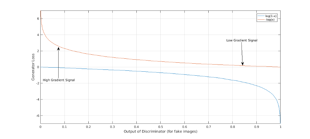
In practice we can perform gradient descent on everything by adjusting the proper signs. A detail taken care in the code that we shall not deliberate more except the fact that doing so improves training. This is by nature of the loss function where performing gradient ascent would mean lower gradients far away from the optimal but high around the optimal. This is not ideal since we would want the exact opposite behaviour for faster convergence. This problem is resolved if gradient descent is performed by modifying the loss function appropriately.

This concludes the description of GAN — concept, architecture, loss function and how does training traverses through the loss landscape. But let us recapitulate our original intention, which is to sample from a distribution without explicitly knowing the distribution. So far, we have convinced ourselves that the loss function and training process discussed above mathematically formalise the dynamics of the adversarial game played between the discriminator and generator. In the next section we would convince ourselves that playing the game does unsure proper sampling.

How does playing a game satisfy our sampling requirements

In the previous section, we first understood the intuition and then the maths. In this section, let’s do the opposite here.

Let’s revisit the loss

To express the expectation in terms of the distribution we have

Now,

Note here that this inverse is strictly not an inverse (the inverse does not exist if we use ReLU), however we abuse notation here a bit and assign inverse G(z) to be any function that given an image spits out a latent variable of the same distribution as z.

Moving forward, if we know the distribution of z, and we know that it transforms(continuously) to an image, we can also express the distribution of all images that is generated by all possible values of z. Remember, that it is this distribution that we want to match with the distribution of images in our training set. Let’s call that p$_g$(x).

Let’s re-write our loss function once again and make the above substitution

maximising the loss in terms of the discriminator function we get

Thus given a G, we get the optimal D as D*(x)

Putting the optimal D* back to the Loss function (which we then have to minimise), we have

multiplying and dividing each term under the integral by 2, we get

Since KL divergence is a strictly positive number. Intuitively it is also the measure of similarity between two distributions. The minimum value of the integral is obtained when,

We therefore prove that the two-player game and the associated loss function does end up in a generator whose output matches the distribution of the real images in the data-set.

You may wonder that what is so special about this strategy though, that produces such amazing results. Let’s look at another toy example to illustrate this edge that GANs enjoy compared to traditional maximum-likelihood approach.

You may wonder that what is so special about this strategy though, that produces such amazing results. Let’s look at another toy example to illustrate this edge that GANs enjoy compared to traditional maximum-likelihood approach.

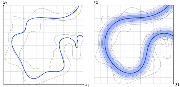
In this image, we are looking at a simplified case with just two dimension. Let us assume that our required distribution is actually the squiggly blue line. By design, traditional maximum likelihood methods assigns a finite probability density to all the real image examples it sees so it tends to smear out the probability mass smoothly around the mean to regions which does not qualify as a legitimate natural image. In effect it misses the nooks and crannies of the real distribution. It is too smooth. GANs don’t have these restrictions. All it needs to do is to win the game between the discriminator and the generator by latching on to some subset (with a degree of variability) around the training examples it sees.

Ending Note

In this article we attempted to understand the mechanism of GANs in a hybrid fashion that involved lots of intuition, code snippets and hand-wavy maths. Unfortunately like most things in life GANs also have convergence issues that were not discussed in this article. Here is a nice article about that.

Over the short-span of 5 years since its inception, the research community have proposed several modifications to improve overall GAN convergence and certain modification to tailor towards specific tasks. You should totally check this repository out which lists the most popular GANs developed till date.

Thanks for reading. Hope you learnt something cool today. :) Till next time.

References

1. https://www.thispersondoesnotexist.com/
2. https://www.thispersondoesnotexist.com/
3. Generative Adversarial Networks, Ian J. Goodfellow, Jean Pouget-Abadie, Mehdi Mirza, Bing Xu, David Warde-Farley, Sherjil Ozair, Aaron Courville, Yoshua Bengio. https://arxiv.org/abs/1406.2661
4. https://github.com/ageron/handson-ml2/blob/master/17_autoencoders_and_gans.ipynb
5. http://cs231n.stanford.edu/
6. http://introtodeeplearning.com/